Conservative Fields: Examples

In my previous post on the basic theory behind conservative vector fields, I described some of the mathematical properties these fields will have:

- A conservative field has no curl:    

- By extension, a vector of 3 components (Mi + Nj + Pk) can be checked for conservancy with a component test:

            

- A conservative field can be 'integrated' to find a potential function. Conversely, any gradient of a function is conservative: 

This is all good stuff, but I like to see visual examples whenever possible. When we're talking graphs of vector fields and functions in space, this is entirely possible! I'm going to go through some examples now, using the graphs to emphasize the math.

For this post, I'll be staying with 2-dimensional vectors in the x-y plane. We can still write a 2-d vector as (xi + yj + 0k) when necessary--if the cross product has to be evaluated, for example. The importance of using 2-d vectors, however, is that it allows me to graph the potential function, rather than simply graphing the level curves of that function. Scalar functions of 3 variables are tough to visualize. Anyway, on with the show!

Gravity: A Central Force

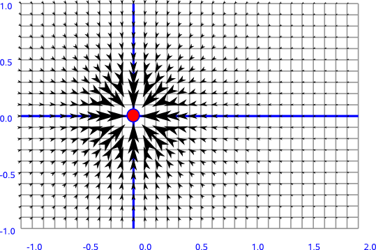
I'll start with a toss-up, the force field of gravity. This is probably the most-used example of a conservative field ever, but it still has a cool-looking potential function. Newton's Law of Universal Gravitation is given in vector form as:

Here, r is the position vector between point 1 and point 2. (We are dealing with point masses here, a useful approximation). G, m1 and m2 are all scalar parameters that I don't really care about now, so I'm just going to ignore them--they don't change the way the functions will look. By changing the unit vector into its constituent parts, the vector function looks like this:

Graphically, the nature of the force is easy to see. It's also pretty easy to imagine that this force is conservative. Since it's such a common example of a conservative force, I'm not going to bother with any component tests.

Image from www.euclideanspace.com; Maple failed me on this one.

An important note: Gravity is what's called a central force. Central forces have 2 main characteristics:

- They are always oriented towards a central point.

- Their magnitude varies only as a function of distance from this point. 

Springs are another common central force. Anyway, the main idea is that central forces are always conservative. This fact is extremely important in the study of dynamics.

Gravitational potential. This one I made in Maple.

The potential function for the field I used above is given by:

                       

However, the actual gravitational function is defined to be negative. (I'm not exactly why, hopefully I can figure it out later). Anyway, the graph of the gravitational potential function is shown at right. Since we're modeling point masses, the function goes to negative infinity and the mesh breaks down at the origin. 

An important feature of potential functions are 'areas of equal potential:' spots on the graph that share the same potential. These are called equipotential, or level, curves and surfaces. This is a 2-dimensional example, so this function's level curves are circular contours. In three dimensions, the level surfaces of equipotential would be spherical. 

Something A Bit More Contrived

It is not always so simple to observe whether a field is conservative or not, particularly in the cases of fluid flows or complicated electrical fields. Here's a vector function I made up:

Here is its field plot. In this case, it seems that there might be some 'whirlpool' action happening on the left and right sides. Tough to be positive, though. This is where the component test comes in.

Since this vector field does not have a z-component, the other two component tests are trivial.

Pass! We have a conservative field on our hands, appearances to the contrary. The potential function is then: 

With p for potential, of course. (Seriously, how hard is that, you textbook writers?) Take a moment to try and visualize the gradient that results from this function--it does indeed match up to the vector field plotted above.

(Remember, the gradient points in the direction of a function's greatest increase).

Time for a Counter-example

Any bets on whether this one will be conservative or not? 

The graph doesn't really look that different from the previous one, although there are some heavier indicators of curl off to the right. In any case, we can quickly find out that this field does indeed fail the component test:

So there's not cool potential function to look at, and finding the work through this field will be a lot tougher than usual. One thing we can do here is find the actual value of the curl. Letting the z-component equal zero;

With the curl entirely in the k (z) direction, out of the screen. This lines up with what we see above: There is no curl at the origin, but quite a lot at the corners of the graph. It always pays to check for meaning in the math you're doing.

I currently don't know why exactly a non-conservative field won't yield a potential function. This is a topic I will come back to later, whenever I decide to do a more complete discussion on vector calculus. For now, it'll be back to particle dynamics, which is much more fun.